KNN既可以做回归,也可以做拟合,这里只讲回归
模型1
直观地说,给定训练集,对于1个新实例,在训练集中找到最近的k个实例,看这k个实例属于哪一类,判断这个新实例也属于这一类。
KNN模型有3个基本要素:距离,K值,投票规则。
1. 距离
参见范数、测度和距离
根据数据特征,可以是曼哈顿距离、欧氏距离、闵可夫斯基距离。
2. K值
- K太小时,容易过拟合。
- K太大,误差也会很大。
3. 投票规则
多数表决规则(majority voting rule)
误分类概率为$P(Y \neq f(X))=1-P(Y=f(X))$
经验风险为$1/k \sum\limits_{i \in N(k,x)}I(y_i \neq c_j)=1-1/k \sum\limits_{i \in N(k,x)}I(y_i = c_i)$
在某些假设下,$\sum\limits_{i \in N(k,x)}I(y_i = c_i)$最大就是多数表决规则,它等价于经验风险最小。
算法
1. 线性扫描
linear scan
要计算每个新的instance与train set中每个instance的距离。
计算量非常大($O(N_{instance})$)
2. kd树2
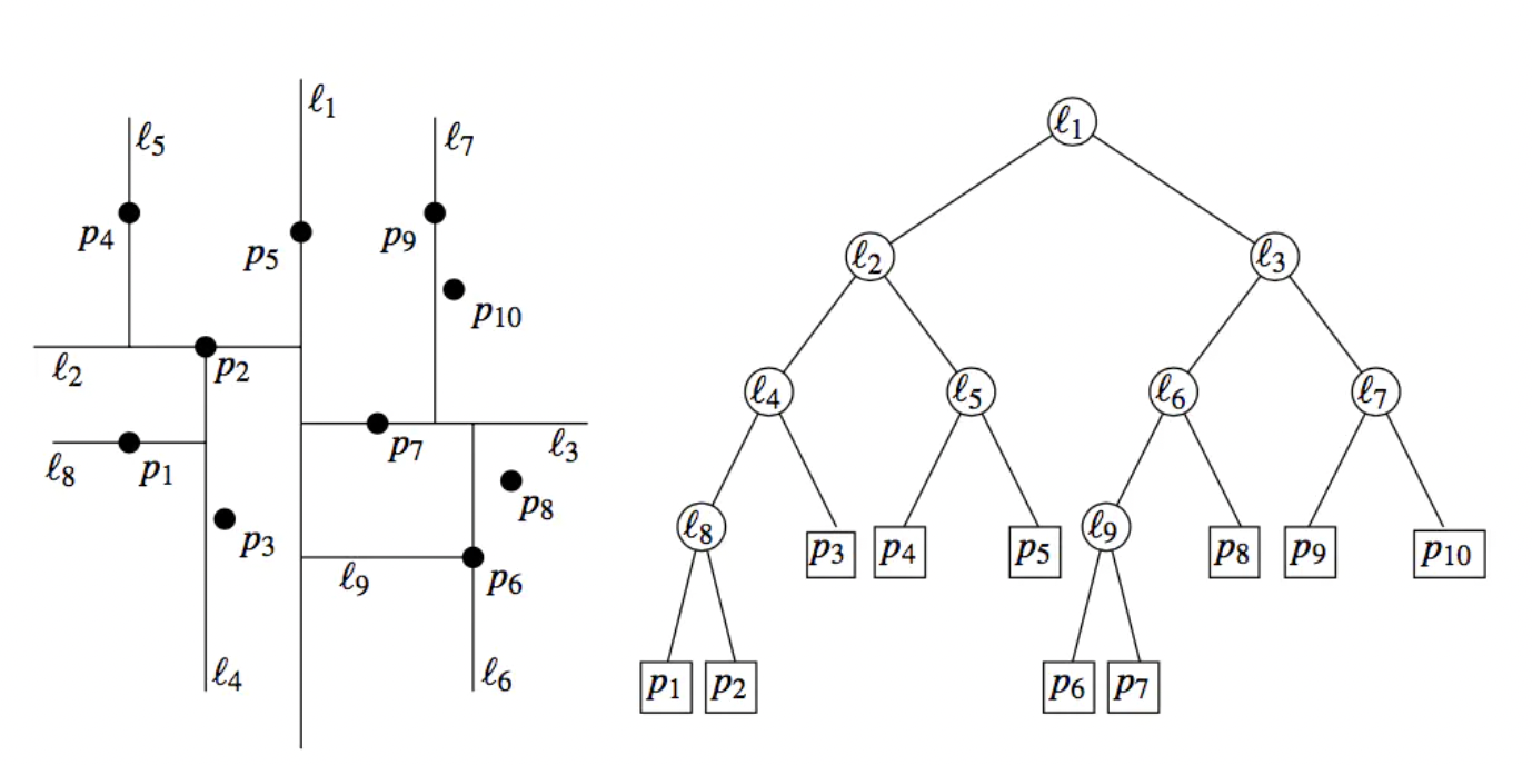
为了减少计算量,引入二叉树算法。
首先生成kd树,然后用kd树找到最近的点。
2.1 生成kd树3
输入:train set
输出:kd树
递归:对于深度为j的节点,选择$x_l$作为切分的坐标轴 ($l=j \mod k +1$)
以$x_l$的median作为切分点,生成深度为j+1的2个子节点。
左子节点小,右子节点大。
递归,直到所有的点全部切分完毕。
2.2 搜索kd树
输入:kd树,目标点x
输出:x的最近邻
step1:找到包含x的叶节点。(从根节点递归向下搜索)
step2:nearest=此叶节点,nearest_length=x和nearest的距离
step3:向父节点回退
step4: 当前节点进行2个操作:
- 如果当前节点与x的距离,比nearest_length小,那么nearest=此叶节点,nearest_length=x和nearest的距离
- 如果以x为圆心,nearest_length为圆心的圆,与兄弟节点矩形相交,那么搜索兄弟节点
step5:转到step3,直到退回到根节点。nearest就是要找的x的最近邻点。
算法评价:
- 如果点是随机分布的,复杂度为$O(\log N)$
- 维度越大,复杂度越高,当维度接近实例数时,效率接近线性搜索。
sklearn实现
from sklearn import neighbors, datasets

iris = datasets.load_iris()
X = iris.data[:, :2]
y = iris.target
clf = neighbors.KNeighborsClassifier(n_neighbors=15, weights='uniform')
clf.fit(X, y)
KNeighborsClassifier(algorithm=’auto’, leaf_size=30, metric=’minkowski’,metric_params=None, n_jobs=1, n_neighbors=15, p=2,weights=’uniform’)
一个完整的例子
这个例子来自CDA课程4
import numpy as np
import matplotlib.pyplot as plt
from matplotlib.colors import ListedColormap
from sklearn import neighbors, datasets
n_neighbors = 15
iris = datasets.load_iris()
X = iris.data[:, :2]
y = iris.target
h = .02 # step size in the mesh
# Create color maps
cmap_light = ListedColormap(['#FFAAAA', '#AAFFAA', '#AAAAFF'])
cmap_bold = ListedColormap(['#FF0000', '#00FF00', '#0000FF'])
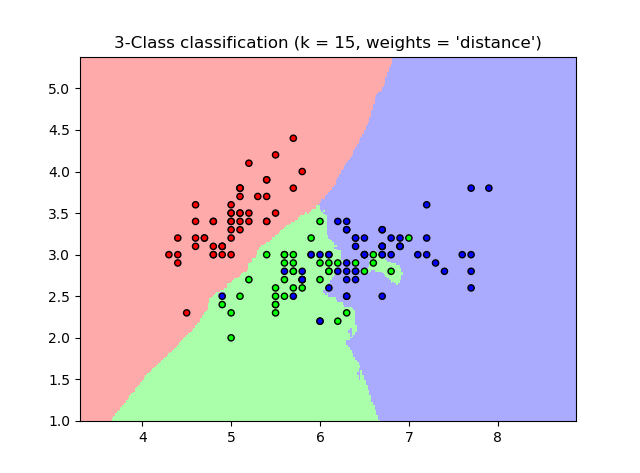
for weights in ['uniform', 'distance']:
# we create an instance of Neighbours Classifier and fit the data.
clf = neighbors.KNeighborsClassifier(n_neighbors, weights=weights)
clf.fit(X, y)
# Plot the decision boundary. For that, we will assign a color to each
# point in the mesh [x_min, x_max]x[y_min, y_max].
x_min, x_max = X[:, 0].min() - 1, X[:, 0].max() + 1
y_min, y_max = X[:, 1].min() - 1, X[:, 1].max() + 1
xx, yy = np.meshgrid(np.arange(x_min, x_max, h),
np.arange(y_min, y_max, h))
Z = clf.predict(np.c_[xx.ravel(), yy.ravel()])
# Put the result into a color plot
Z = Z.reshape(xx.shape)
plt.figure()
plt.pcolormesh(xx, yy, Z, cmap=cmap_light)
# Plot also the training points
plt.scatter(X[:, 0], X[:, 1], c=y, cmap=cmap_bold,
edgecolor='k', s=20)
plt.xlim(xx.min(), xx.max())
plt.ylim(yy.min(), yy.max())
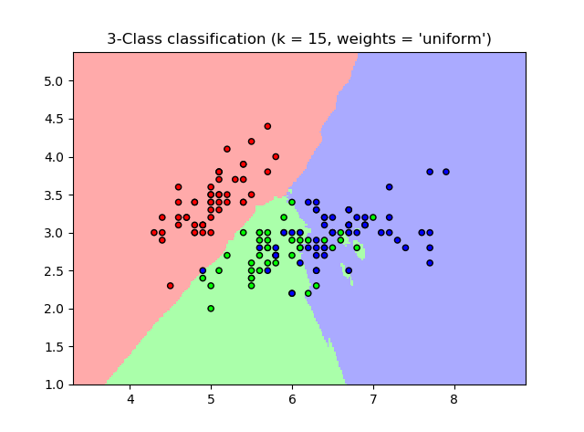
plt.title("3-Class classification (k = %i, weights = '%s')"
% (n_neighbors, weights))
plt.show()
这个图可以用于很多分类模型(二维)